Maneuver Calculator
The Maneuver Calculator computes optimal continuous-thrust profiles for orbital maneuvers. Given a spacecraft's current (or live) state and a target orbit, it solves for a thrust arc sequence that minimises fuel for the transfer time, then lets you verify the result through a dynamics simulation before committing it to the main scenario. It integrates directly with the Constraint Monitor: once a correction is requested, the initial and final boundary conditions are pre-filled automatically.
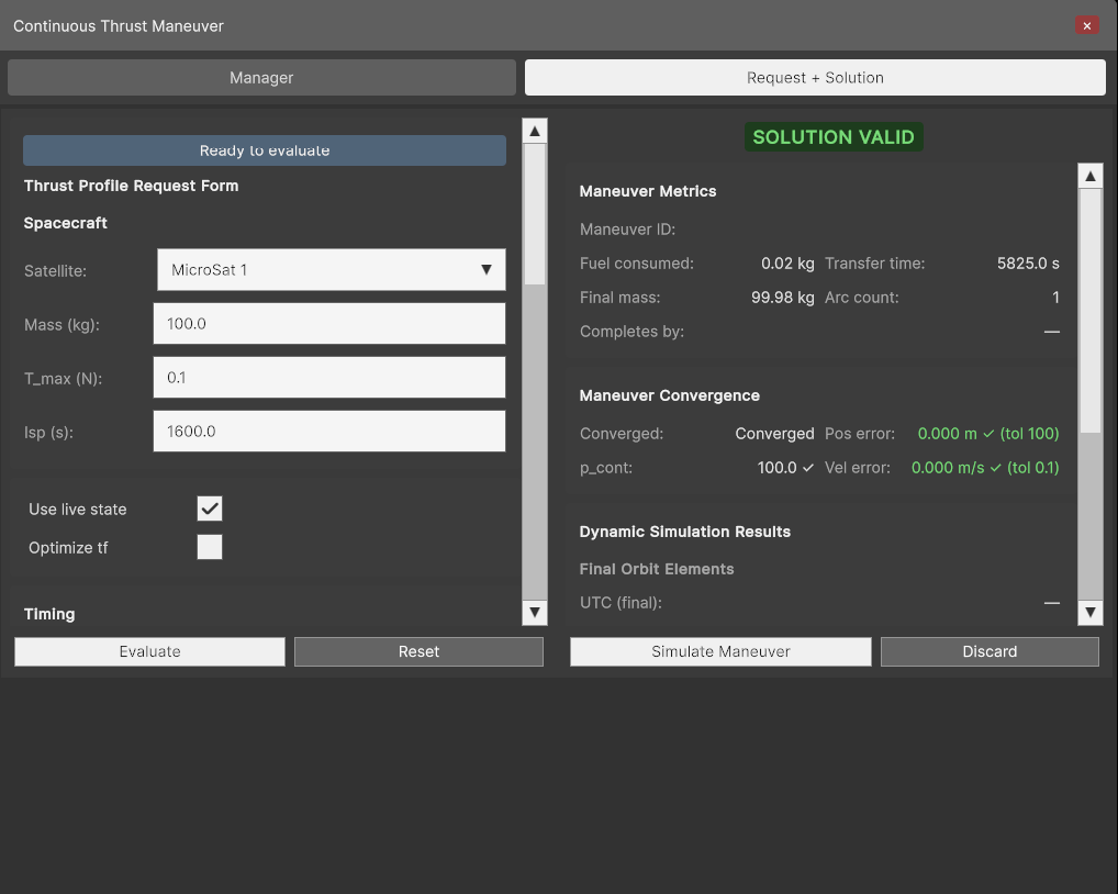
Use cases
- Station-keeping corrections — compute a raise/lower maneuver when a constraint violation is detected or predicted.
- Constellation slot maintenance — correct in-track or cross-track drift for formation-flying satellites.
- Orbit transfer design — evaluate fuel and time cost for a target orbit before committing to execution.
- What-if analysis — run a branched scenario to compare the maneuvering satellite against the unperturbed fleet without touching the main simulation.
- Batch maneuver management — store, export, and reload maneuver plans across sessions.
Typical workflow
- Fill Thrust Profile Request Form manually or via violation in the Constraint Monitor and click Request correction.
- Confirm initial/final Kepler elements and spacecraft parameters (mass, T_max, Isp).
- Set Duty Cycle (maneuver completion time) and Click Evaluate.
- If the Maneuver Calculator returns a solution, review the metrics and convergence stats.
- To dynamically verify the maneuver, click Simulate Maneuver to open Maneuver Propagation Setup.
- Attach the maneuver to the satellite and choose Branched Fleet Scenario to perform a propagaton that will not impact the main scene.
- Configure propagation settings and click Run and review the final orbit elements and Constraint Monitor Review in the solution panel.
Theory
The solver uses indirect optimal control based on Pontryagin's Minimum Principle (PMP) [^1]. Given fixed initial and final orbital states, the problem is cast as a two-point boundary value problem (TPBVP): the spacecraft state (position, velocity, mass) is pinned at both ends, and the solver finds the costate (adjoint) variables — most importantly the primer vector whose direction dictates where the thruster must point at every instant to minimise fuel consumed. PMP shows that the fuel-optimal throttle is bang-bang: the engine is either fully on or fully off, switching when the primer vector magnitude crosses a threshold.
Because bang-bang trajectories have hard on/off discontinuities, a standard Newton-based solver cannot converge to them directly. The solver uses a sigmoid continuation strategy [^2]: the hard switch is replaced by a smooth sigmoid that is gradually sharpened across a schedule of seven steps (p = 0.01 → 100). Each step warm-starts from the previous solution, walking smoothly from an always-thrusting arc to the true bang-bang profile. At each continuation step the TPBVP is solved by Lobatto IIIa collocation — the trajectory is discretised on an adaptive mesh and the ODE residuals are enforced simultaneously across all nodes, making the method far more robust to costate sensitivity than single-shooting.
[^1]: Bryson, A. E. & Ho, Y. C. (1975). Applied Optimal Control: Optimization, Estimation and Control. Taylor & Francis.
[^2]: Bertrand, R. & Epenoy, R. (2002). New smoothing techniques for solving bang–bang optimal control problems — numerical results and statistical interpretation. Optimal Control Applications and Methods, 23(4), 171–197.
Window overview
The Continuous Thrust Maneuver window has two tabs: Manager and Request + Solution.
Request + Solution tab
Thrust Profile Request Form (left panel)
- Satellite — Spacecraft to maneuver. Pre-populated when opened from the Constraint Monitor.
- Mass (kg) — Spacecraft wet mass at maneuver start.
- T_max (N) — Maximum available thrust.
- Isp (s) — Specific impulse of the thruster.
- Use live state — When checked, the current simulation state is used as the initial condition. Uncheck to enter a manual initial state.
- Optimize tf — When checked, the solver searches for less fuel-costly solutions by varying flight time.
- t_start (JD) — Maneuver start Julian Date.
- Duty Cycle — Fraction of orbital period to compute flight time that auto-fills t_flight (s).
- Initial Kepler Elements — Initial satellite state to solve from, auto-filled by the Use live state toggle.
- Desired Δ Kepler Elements — Desired change in Kepler Elements.
Click Evaluate to run the solver. Click Reset to clear the form back to defaults.
Solution panel (right panel)
Once the solver completes, the right panel updates with:
- Status — Solution status messages.
- Maneuver Metrics — Thrust profile's estimated fuel consumed, final mass, transfer time, arc count, and estimated completion UTC.
- Maneuver Convergence — Converged flag, p_cont (bang-bang control parameter), position error vs. tolerance, velocity error vs. tolerance.
Click Simulate Maneuver to open the Maneuver Propagation Setup and run a full dynamics check — this populates the remaining sections of the solution panel. Click Discard to discard the current solution without saving it.
Maneuver Propagation Setup
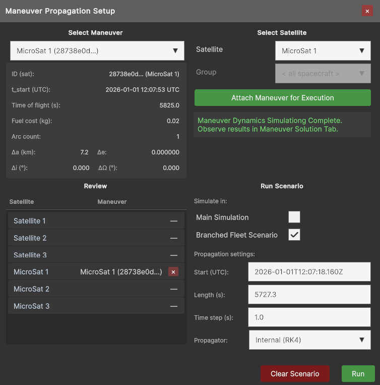
Maneuver Selection (left panel)
Choose a maneuver from the dropdown. The panel shows a summary of the selected plan:
| Field | Description |
|---|---|
| ID (sat) | Shortened maneuver ID and originally chosen satellite for maneuver. |
| t_start (UTC) | Planned maneuver start time. |
| Time of flight (s) | Total burn duration. |
| Fuel cost (kg) | Propellant consumed. |
| Arc count | Number of thrust arcs in the profile. |
| Δa / Δe / Δi / ΔΩ | Predicted orbital element changes. |
The Review table at the bottom lists every satellite in the fleet and shows which maneuver (if any) is assigned to each one. Click the red × next to an assignment to remove it.
Satellite Selection and Propagation Settings (right panel)
Select the target spacecraft and click Attach Maneuver for Execution to assign the loaded maneuver to that satellite. A status line confirms when the assignment is active.
Run Scenario
Configure the propagation run:
| Setting | Description |
|---|---|
| Main Simulation | Execute the maneuver in the live simulation (modifies the running scenario). |
| Branched Fleet Scenario | Run a copy of the fleet in the background, leaving the main simulation untouched. Recommended for analysis. |
| Start (UTC) | Propagation start timestamp. |
| Length (s) | Total propagation duration. |
| Time step (s) | Integration step size. |
| Propagator | Numerical integrator (e.g. Internal RK4/TUDAT/SGP4). |
Click Run to execute. Once complete, the Request + Solution tab's Dynamic Simulation Results and Constraint Monitor Review sections are populated. Click Clear Scenario to reset all assignments before starting over.
Dynamic Simulation Results and Constraint Monitor Review
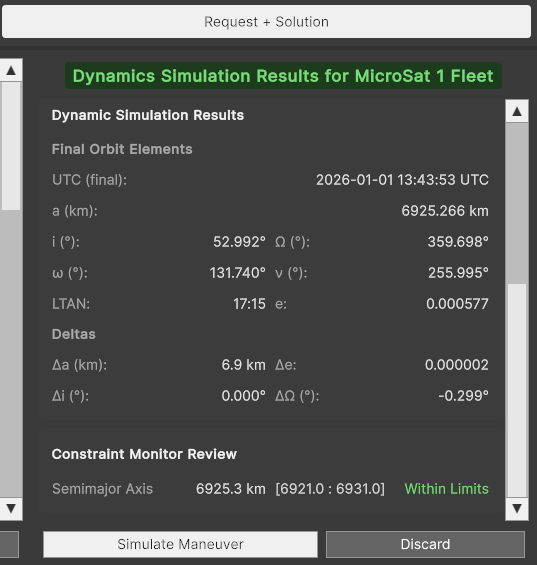
After the branched simulaton propagation run completes, the solution panel shows Final Orbit Elements, change in Kepler Elements and Constraint Monitor's results review.
Manager tab — Stored Maneuvers
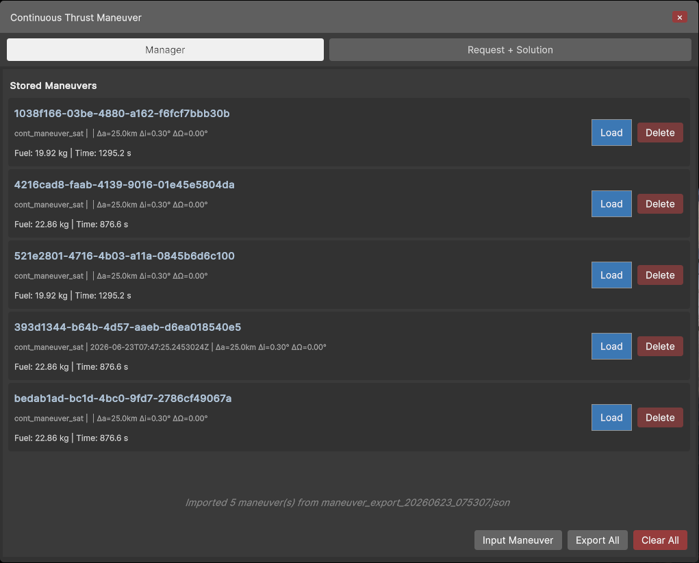
The Manager tab lists all maneuver plans currently held in memory. Each entry shows:
- Maneuver Identifier
- Target satellite name
- Orbit deltas: Δa (km), Δi (°), ΔΩ (°)
- Fuel cost (kg) and transfer time (s)
| Button | Action |
|---|---|
| Load | Load the selected maneuver into the Request + Solution tab for review or editing. |
| Delete | Remove the maneuver from the stored list. |
| Input Maneuver | Manually enter a maneuver plan from a JSON string. |
| Export All | Save all stored maneuvers to a JSON file (maneuver_export_<timestamp>.json). |
| Clear All | Remove all stored maneuver plans. |
Previously exported plans can be re-imported via Input Maneuver or through the API, making it possible to share maneuver libraries across sessions.
Example
A full worked example demonstrating constraint violation detection, correction request, and maneuver simulation is provided in:
examples/example_constraint_monitor_correction.py